This section is only for those who know a little about neural nets and who desire to look under the hood of our neural indicators. It is complicated, but not at all necessary to understand. The NI can be used just fine if you don’t understand a word of what follows. In the end, the choice of which of the NI to use, like all financial modeling, is more a matter of experimentation, than a matter of science and understanding.  In fact, if you do not understand the following explanations, it will be beyond the scope of our technical support services to teach the material to you. Instead, we must refer you to the "bible" of neural networks for further study:

Rumelhart, D., McClelland, J., and the PDP Research Group.  Parallel Distributed Processing.  Explorations in the Microstructure of Cognition.  (Three volumes.)  Cambridge, MA, The MIT Press, 1987.

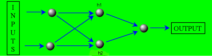
Overview

All neural nets in the Neural Indicators have "input neurons" into which the NeuroShell Trader places the current bar of input values. There are "connections" between each input neuron and each of two "hidden neurons" designated h1 and h1. Each of the two hidden neurons in turn has connections to the single "output neuron". Here is a picture of what the neural network looks like:

Associated with each connection there is a "weight" which the optimizer assigns. The weight is a real number, usually between –1 and 1.

Processing

Input values are placed into the input neurons and then "scaled" according to the window size specified in the "scale" parameter. That makes the values in the input neurons smaller and more normalized.

Next the hidden neurons are computed. To compute h1, each input is multiplied by the weight in the connection leading from that input to h1. If there are 3 inputs, for example, there will be three products. The sum of the three products is placed into h1.

Each hidden and output neuron has an "activation function " associated with it. The activation function is applied to the sum in the neuron to produce a new value to replace the old one. Unless otherwise noted, the activation functions in our nets are the hyperbolic tangent function from trigonometry.

Next, the output neuron is computed. The computation of the output neuron is similar to the computation of a hidden neuron. Each hidden neuron value is multiplied by the weight in the connection leading from that hidden neuron to the output neuron. Since there are two hidden neurons, there will be two products. The sum of the two products is placed into the output neuron. The activation function is applied to the sum in the output neuron to produce a new value to replace the old one. This new value becomes the output of the net.

Most neural networks have additional connections from fixed neurons, and these are called "bias" connections or bias weights. Neural Indicators do not use bias connections so that we can keep the number of weights low. For the vast majority of financial inputs, they are not necessary.

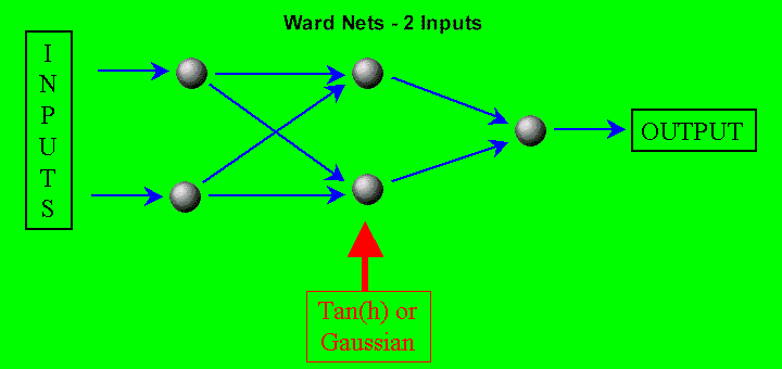
Ward Nets

The distinguishing feature of the Ward Nets is that each of the hidden neurons can have either of two different activation functions.  The use of two different activation functions gives the network two different views of the data and often leads to more accurate signals. Each activation function can be either the hyperbolic tangent, or the Gaussian function exp(-x*x/2.0).  The values of the parameters determine which activation functions are used as explained later. Both neurons can use the hyperbolic tangent, both can use the Gaussian, or there can be one of each.  The optimizer can make the decision for you.

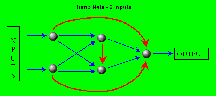
Jump Nets

The Jump Nets always use the hyperbolic tangent activation functions, but they have extra connections with weights. In addition to the connections already mentioned, there are connections from each input neuron to the output neuron. There is also a connection from the first hidden neuron to the second hidden neuron. There are thus more weights in a Jump Net.

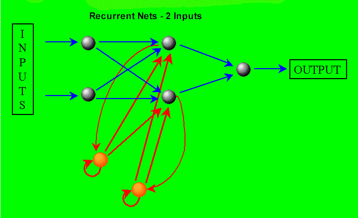
Recurrent Nets

All of the nets except the recurrent nets are "feed forward" nets, meaning the propagation of values through the nets always goes forward. Recurrent Nets, however, also have backwards connections. There are connections from the two hidden neurons to two additional "recurrent neurons" in the "input layer". Data in the recurrent neurons is delayed one bar before it is fed back into the hidden neurons like the inputs are on the next bar.

There are also connections from the recurrent neurons to themselves. In essence, recurrent neurons keep a weighted moving average of the hidden neurons.

The recurrent neurons provide a "memory" of the values that have been in the hidden neurons on previous bars. In this way they are looking back in time, because the memory is fed into the net just as the current inputs are fed. The hidden neurons are a compressed summary of the current bar’s inputs, and so the recurrent nets are a compressed summary of the last several bars of inputs.

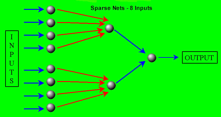
Sparse Nets

These nets have either 2, 3, or 4 hidden neurons, but any given input is only connected to one hidden neuron. All hidden neurons are connected to the output neuron, however. The lack of hidden neurons connected to various combinations of inputs means that some relationships may be lost. Here is a diagram on one Sparse Net: